In this blog post, I will try to explain the fascinating (but not new) world of Kolmogorov-Arnold Networks (KANs). I will explore how they differ from the more commonly known Multi-Layer Perceptrons (MLPs), discuss their strengths and weaknesses, and provide examples to illustrate their applications.
What are Kolmogorov-Arnold Networks?
Kolmogorov-Arnold Networks are named after the Kolmogorov-Arnold representation theorem. This theorem states that any continuous function of several variables can be represented as a superposition of continuous functions of one variable and addition. This powerful idea forms the basis of KANs, which aim to represent complex functions using simpler, univariate functions and summation operations.
Too difficult? Let’s break it down!
Explanation Level 2
Imagine you have a complex machine that takes several inputs (like a multi-variable function). The theorem tells us that we can break down this complex machine into simpler machines (each taking only one input) and then combine their outputs to get the same result as the original complex machine.
Explanation Level 3
Think of baking a cake. The final cake (the complex function) is a result of several ingredients mixed together. According to the theorem, you can imagine creating the cake by first processing each ingredient separately (simple functions) and then combining them in a certain way to get the final product.
Differences from Multi-Layer Perceptrons (MLPs)
While both KANs and MLPs are types of neural networks, they have some key differences:
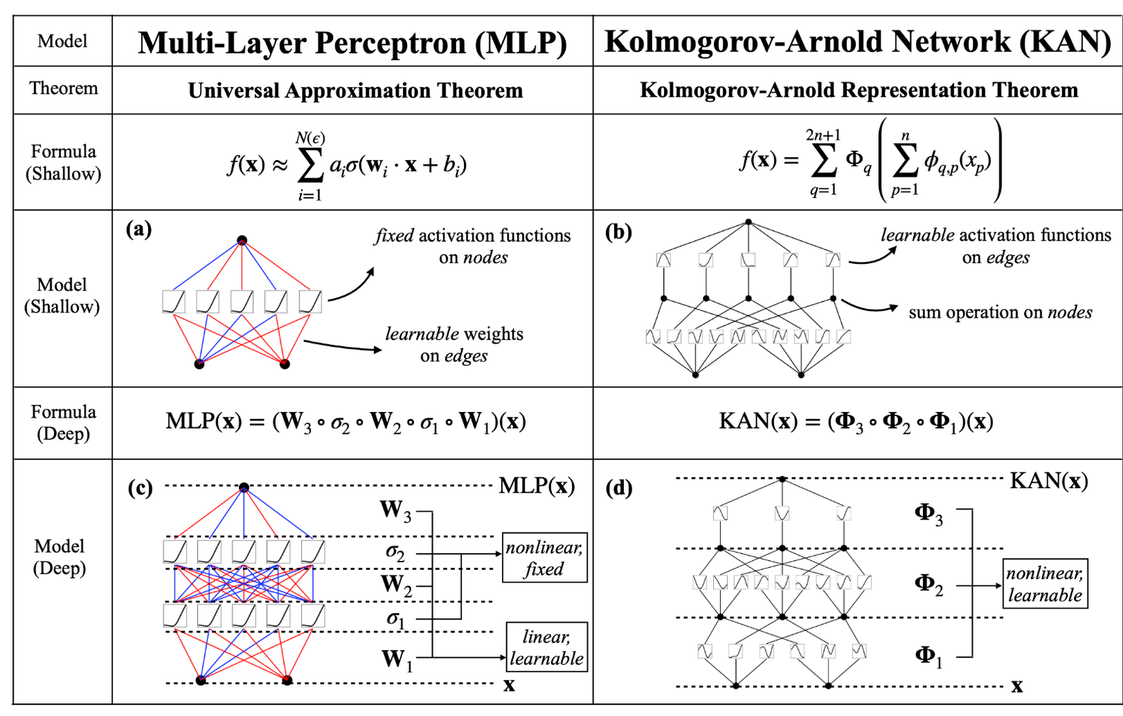
- Representation Theorem: KANs are based on the Kolmogorov-Arnold representation theorem, focusing on decomposing multivariate functions into univariate functions. In contrast, MLPs are based on layers of neurons with nonlinear activation functions that aim to approximate complex functions through a hierarchical structure.
- Network Structure: KANs typically use fewer parameters because they leverage the decomposition of functions into simpler components. MLPs, on the other hand, often require more layers and neurons to achieve similar levels of function approximation, leading to a larger number of parameters.
- Training Complexity: Training KANs can be more challenging due to their unique structure and the need to optimize the decomposition of functions. MLPs, while also complex, benefit from well-established training algorithms like backpropagation and various optimizers that are widely researched and understood.
- While we have fixed activation functions on nodes and learnable weights on edges, KANs have learnable activation functions on edges and sum operation on nodes.
Why Kolmogorov-Arnold Networks are Good
Pros
- Efficiency: KANs can achieve function approximation with fewer parameters, making them potentially more efficient than MLPs in terms of memory and computational requirements.
- Theoretical Foundation: The Kolmogorov-Arnold representation theorem provides a strong theoretical basis for KANs, ensuring that they can approximate any continuous function.
- Simpler Components: By breaking down multivariate functions into univariate components, KANs can leverage simpler functions, which may lead to better interpretability and understanding of the network’s behavior.
Cons
- Training Difficulty: The unique structure of KANs can make them more difficult to train compared to MLPs. Optimizing the decomposition of functions and tuning the network parameters can be challenging.
- Limited Popularity: KANs are not as widely used or researched as MLPs, meaning there are fewer resources, tools, and community support available for practitioners.
- Specialization: KANs may be more specialized and less versatile than MLPs, which can be applied to a wide range of tasks and problems due to their general-purpose design.
Examples and Applications
To illustrate the power and potential of Kolmogorov-Arnold Networks, let’s look at a few examples and applications:
Example 1: Function Approximation
Consider the problem of approximating a complex, multivariate function f(x, y, z) . Using a KAN, we can decompose this function into univariate functions g_i and combine them using summation:
$$f(x, y, z) \approx \sum_{i=1}^n g_i(h_i(x) + k_i(y) + l_i(z))$$This decomposition allows us to approximate the original function with fewer parameters and potentially more interpretability.
Example 2: Signal Processing
In signal processing, KANs can be used to decompose and reconstruct signals. By breaking down a complex signal into simpler components, KANs can help in noise reduction, feature extraction, and other signal processing tasks.
Example 3: Control Systems
KANs can be applied in control systems where the goal is to model and control complex, nonlinear systems. The efficiency and theoretical foundation of KANs make them suitable for approximating the system’s behavior and designing appropriate control strategies.
Conclusion
Kolmogorov-Arnold Networks offer a unique (and astonishing!) and theoretically grounded approach to function approximation. While they present some challenges in terms of training and specialization, their efficiency and strong theoretical basis make them a valuable tool in specific applications.
The path to mastering KANs may be less traveled than that of MLPs, but for those willing to explore this fascinating world, the rewards can be significant. Maybe we are at the dawn of a new era in data science, where Kolmogorov-Arnold Networks will play a crucial role in solving complex problems and unlocking new possibilities.
If you have any questions or would like to see more examples, feel free to reach out at matheus.pestana at fgv.br :)!